Climate Distortion in ACORN-SAT

Author: Dr. Michael Chase

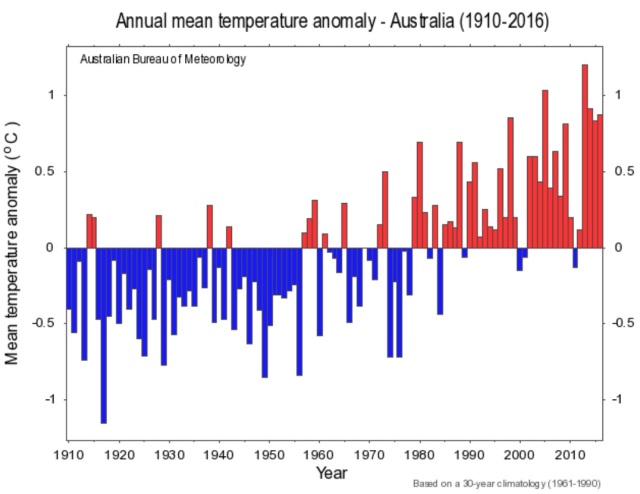
Source of the figure above: http://www.bom.gov.au/climate/change/#tabs=Tracker&tracker=timeseries

Summary

There is considerable climate distortion in the ACORN-SAT version of surface air temperatures of Australia from 1910 to present, with most of the distortion in the first half of the 20th century. The main problem lies in the assumption made that all non-climatic influences, detected via anomalous step changes in temperature, do not vary with time. Many non-climatic influences, such as urban heating and screen degradation, do vary with time, so whilst the ACORN-SAT correction process does a good job for some years before step changes occur, it over-corrects at earlier times, often giving an invalid cooling of the early decades of the 20th century.

This problem with ACORN-SAT is only at the final stage of processing, when corrections are applied. The step change information itself is highly valuable and it should be possible to produce a more accurate version of the temperature history of Australia, if possible by following how non-climatic influences vary with time in the data, or by modelling.

Introduction

Reconstructing the actual surface temperatures of Australia back to 1910 is a difficult job which has to contend with several non-climatic influences on what is sometimes incomplete, erroneous and poorly documented temperature data. The ACORN-SAT reconstruction detects non-climatic influences when they change, either sudden onsets or removals. Data from neighbouring stations is used to detect and estimate the size of sudden and persistent changes in relative temperature, deemed to be non-climatic in origin. The final stage of processing is to correct the temperature data so as to reveal the true background climate variations.

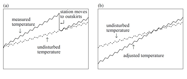
The following figure illustrates where things go wrong for any time-varying influence, shown as the red curve:

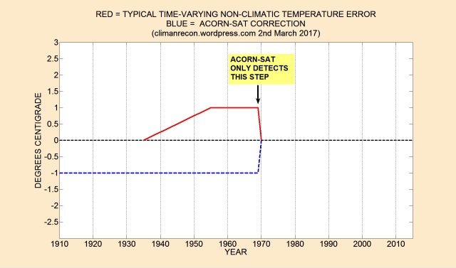
The red curve in the figure above applies to common non-climatic influences such as urban growth around weather stations located in towns, or the gradual degradation of the thermometer screen. When a weather station moves out of town, or to a better location within the town, or a screen is replaced, the temperatures recorded suddenly drop (relative to those of neighbours), an event detected by the ACORN-SAT algorithms. The erroneous assumption (shown as the blue curve) is then made that the non-climatic influence is constant in time, resulting in over-correction in the entire period leading up to the full effect of the influence.

Examples

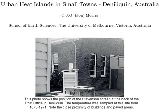
Source of the picture above: http://www.hashemifamily.com/Kevan/Climate/Heat_Island.pdf

When the weather station at Deniliquin moved to a better location in the town in 1971, the minimum temperatures recorded fell by around 1 degree C on average, probably mostly due to the removal of the heating effect of the buildings and paving stones. ACORN-SAT assumes that the urban heating in 1971 was constant all the way back to 1910.

Another example is given in the ACORN-SAT documentation itself, for a site move in Inverell in 1967:

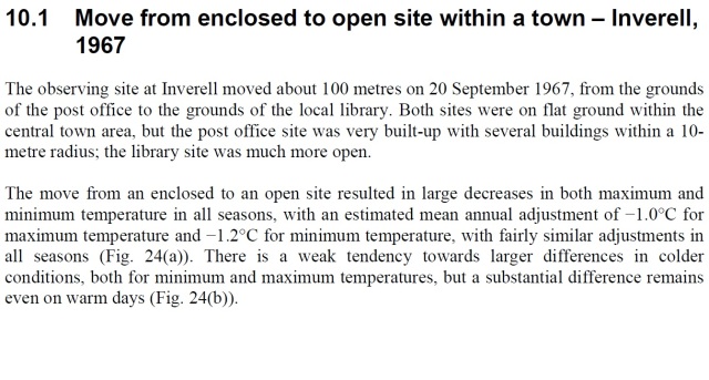
Source of the extract above: http://cawcr.gov.au/technical-reports/CTR_049.pdf

Again, ACORN-SAT assumes that the urban heating of the very built-up post office site applied all the way back to 1910, though in this case there were also earlier step changes. Integrating the step changes of time varying influences does not in general get you anywhere near the right answer for early decades.

There are many examples in the ACORN-SAT station adjustment summary of step changes due to equipment replacement, many likely to be due to a recent degradation being removed by the provision of new equipment. ACORN-SAT assumes that the degraded equipment was in place all the way back to 1910.

Previous Commentary

I must apologise at this stage for being unfamiliar with most of the literature on temperature homogenisation, so am probably not giving due credit to previous authors. The following two examples are relevant, firstly from Hansen et al, 2001:

Source of the figure above: https://pubs.giss.nasa.gov/abs/ha02300a.html

The figure above shows a time-varying urban heating being correctly removed around the time of a station move, but being over-corrected at earlier times. There are several examples in ACORN-SAT of town data being merged with that from an airport, with an unknown amount of historical urban heating being turned into erroneous cooling of early data.

The second example is from Stockwell and Stewart (2012), correctly identifying a major reason why the pre-cursor to ACORN-SAT gives more apparent warming than is found in raw data:

Source of the figure above: http://citeseerx.ist.psu.edu/viewdoc/download?doi=10.1.1.362.9661&rep=rep1&type=pdf

The Way Forward

ACORN-SAT only falls at the final hurdle, the temperature step changes that it identifies can be used to redeem it. Here is an example of a validation of one of its discontinuities:

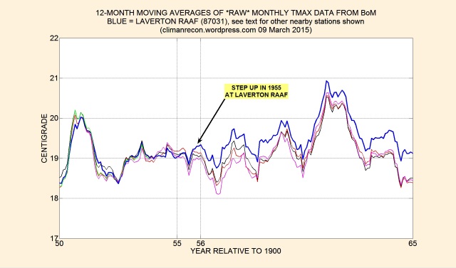
The figure above shows an anomalous step-up in average maximum temperatures at Laverton RAAF (blue curve), as well as possible indications of anomalous warming in the 1960s relative to neighbours: Melbourne Regional (-0.8C), Essendon Airport (-0.1C), Black Rock, and Tooradin.

One way to deal with urban warming, most of which is historical rather than current, is to construct composite temperature records, in the example above following Laverton up to its step change, then jumping to a suitably scaled average of its more rural neighbours.

For large temperature step changes, such as those shown above for Deniliquin and Inverell, it should be possible to follow, and thereby properly correct, the time variation of the urban warming down to a certain minimum level. For smaller temperature changes, many of which occur in regions without reliable near neighbours, modelling of the urban heating can be used, guided by any available documentation of the station history.

This post ends here, examples will be shown in later articles of the size of ACORN-SAT errors, but the focus will shift to the question of what is the right answer for Australian temperature histories.